We recently published the hadron package on CRAN. You may install it
via install.packages("hadron"). Here we explain how to use hadron
to analyse so-called correlation functions from Monte Carlo
simulations in particle and statistical physics.
Data Type cf for Correlation Functions
In the following we will discuss the analysis of so called correlation functions. We denote a Markov Chain Monte Carlo ensemble as \(U=\{U_\tau\}\), where each \(U_\tau\) has additional internal indices, in particular space \(x\) and Euclidean time \(t\). Consider a set of observables \(O_i[U]\), for which one can compute correlation functions \[ C_{ij}(t - t')\ =\ \langle \sum_x O_i[U](x, t) | \sum_x O_j[U](x, t') \rangle\,, \] where \(\langle . \rangle\) denotes the expectation value over the Markov chain ensemble.
For instance in Lattice QCD, but also for other physical theories one can show that \[ C_{ij}(t) \propto \sum_n A_{ni} A_{nj} e^{- E_n t}\,. \] \(E_n>0\) are real values energy levels and the \(A_{ni}\) amplitudes.
The hadron package provides a data type or better a class for such
correlation functions and correlation matrices, which is called
cf. There is a whole list of input
routines available to import data from HDF5, text or binary formats
into the cf container. The most important ones are compiled
in the following table:
| Hadron Function | Correlator Format |
|---|---|
| readtextcf | text |
| readbinarycf | binary, HDF5 |
| readbinarysamples | binary |
| — | — |
For even more flexibility there is the raw_cf container, for
which we refer to the documentation.
In oder to solve the generalised eigenvalue problem (GEVP)
(Michael and Teasdale 1983; Lüscher and Wolff 1990; Fischer et al. 2020)
one has to read several correlation functions into one cf correlator
matrix. For this purpose the combine operation c is defined
for the class cf. Thus, for instance the following code
snipped can be used:
Time <- 48
correlatormatrix <- cf()
for(i in c(1:4)) {
  tmp <- readbinarycf(files=paste0("corr", i, ".dat"), T=Time)
  correlatormatrix <- c(correlatormatrix, tmp)
}
rm(tmp)
This code snippet reads a correlator matrix with four correlation functions from four files. The read functions can also directly read from a list of files. File lists can be created conveniently using the following routines
getorderedfilelist <- function(path="./", basename="onlinemeas",
                               last.digits=4, ending="")
getconfignumbers <- function(ofiles, basename="onlinemeas",
                             last.digits=4, ending="")
getorderedconfigindices <- function(path="./", basename="onlinemeas",
                                    last.digits=4, ending="")
for which we refer to the documentation.
Resampling Strategies
Once the bare data is available as a cf, one has to decide
for an error analysis strategy. This can be either the bootstrap or
the jackknife. To demonstrate this we first load the sample
correlation matrix provided by hadron
data(correlatormatrix)which corresponds to a \(2\times 2\) local-fuzzed correlator matrix with quantum numbers of the pion. First the resampling needs to be performed, for instance for the (blocked) bootstrap
boot.R <- 150
boot.l <- 1
seed <- 1433567
correlatormatrix <- bootstrap.cf(cf=correlatormatrix,
                                 boot.R=boot.R,
                                 boot.l=boot.l,
                                 seed=seed)
Analogously, jackknife.cf initiates the jackknife
resampling. boot.R is the number of bootstrap replicates,
boot.l the block lentgh. Now, it is also possible to plot the
data with errors
plot(correlatormatrix, log="y",
     xlab=c("t/a"), ylab="C(t)")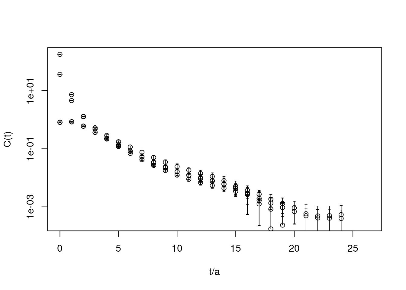
Solving the GEVP
Let us denote the correlator matrix by \(C(t)\). Now we are going to solve the generalised eigenvalue problem \[ C(t)\, v_i(t, t_0)\ =\ \lambda_i(t, t_0)\, C(t_0)\, v_i(t, t_0) \] with some reference time value \(t_0\). One can show that the so-called principal correlators \(\lambda(t, t_0)\) follow for large \(t\)-values the following behaviour \[ \lambda_i(t, t_0)\ \propto\ e^{-E_i(t-t_0)} + e^{-E_i(T-t+t_0)}\,. \] Here, \(T\) is the time extent and we focus on a symmetric correlation matrix in time. However, analogously one can show this with a minus sign for anti-symmetric correlation matrices in time. Of course, we also have \(\lambda(t_0, t_0) = 1\). We re-write the generalised eigenvalue problem by defining \[ w_i\ =\ \sqrt{C(t_0)} v_i \] and solve the simple eigenvalue problem \[ \sqrt{C(t_0)}^{-1}\,C(t)\,\sqrt{C(t_0)}^{-1}\, w_i\ =\ A\, w_i\ =\ \lambda_i(t, t_0)\, w_i \] instead.
In hadron this task is performed as follows on the bootstrap
correlator matrix in the most simple case
t0 <- 4
correlatormatrix.gevp <- bootstrap.gevp(cf=correlatormatrix, t0=t0,
                                        element.order=c(1,2,3,4),
                                        sort.type="values")
Next, the principal correlators \(\lambda_i\) are obtained as follows, where in this case we have \(i=1,2\)
pc1 <- gevp2cf(gevp=correlatormatrix.gevp, id=1)
pc2 <- gevp2cf(gevp=correlatormatrix.gevp, id=2)
plot(pc1, col="red", pch=21, log="y", xlab="t", ylab="C(t)")
plot(pc2, rep=TRUE, col="blue", pch=22)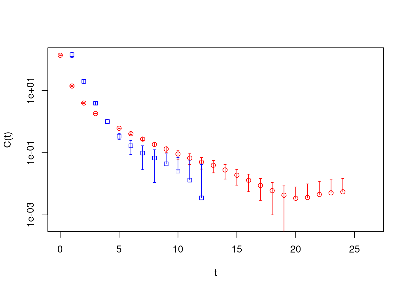
These principal correlators can be analysed as every object of type
cf, see below.
Additional Options
bootstrap.gevp has some additional options which are worth
mentioning.
During the bootstrap procedure for the GEVP, eigenvalues have to be sorted for every \(t\)-value. This can be either done by
values,vectorsordetpassed via the parametersort.type. Whenvectorsis chosen, scalar products of eigenvectors are computed \[ v(t', t_0) \cdot v(t, t_0) \] and the overlap maximised. Whensort.t0is set toTRUE, the comparison time is chosen constant as \(t'=t_0+1\). Otherwise, \(t'=t-1\) is set in dependence of \(t\).With parameter
element.orderthe correlation functions in the input correlator matrix are specified for use in the GEVP. This can be a sub-set of all the correlation functions in the matrix. Double usage is allowed as well.
Extracting Energies
Matrixfit
First, a fit directly to the (principal) correlator can be
performed. The corresponding functionality is provided in
hadron by the function matrixfit and, more modern,
new_matrixfit. Let us discuss here the former in its
application to
pc1.matrixfit <- matrixfit(cf=pc1, t1=6, t2=21, useCov=TRUE,
                           parlist=array(c(1,1), dim=c(2,1)),
                           sym.vec=c("cosh"), fit.method="lm")
## Loading required namespace: minpack.lmplot(pc1.matrixfit, do.qqplot=FALSE,
xlab="t", ylab="C(t)")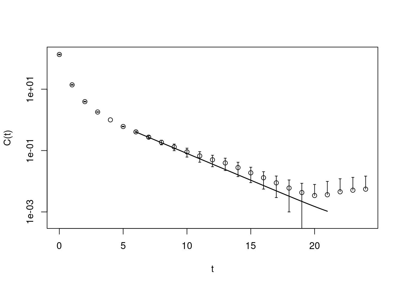
An extended overview is provided by the overloaded summary
function
summary(pc1.matrixfit)
** Result of one state exponential fit **
based on 541 measurements
time range from 6 to 21
ground state energy:
E = 0.4020216
dE = 0.05814395
Amplitudes:
P 1 = 2.997469
dP 1 = 0.4713082
boot.R = 150 (bootstrap samples)
boot.l = 1 (block length)
useCov = TRUE
chisqr = 4.182661
dof = 14
chisqr/dof= 0.2987615
Quality of the fit (p-value): 0.9942633 This yields an energy level with error of \(E =0.402(58)\).
As we know that \(\lambda(t_0, t_0)=1\), we can fit more than a single
exponential to the principal correlator. For this matrixfit
knows the model pc. The corresponding fit model reads
\[
f(t; E, \Delta E, A)\ =\ \exp(-E(t-t_0))(A + (1-A)\exp(-\Delta E(t-t_0))
\]
involving three fit parameters. Of course, the fit must be started at
earlier time slices in order to be sensitive to excited states.
pc1.matrixfit <- matrixfit(cf=pc1, t1=3, t2=20, useCov=TRUE,
parlist=array(c(1,1), dim=c(2,1)),
sym.vec=c("cosh"), fit.method="lm",
model="pc")
plot(pc1.matrixfit, do.qqplot=FALSE,
     xlab="t", ylab="C(t)")
A useful crosscheck is to not plot the raw correlator, but the correlator with the leading exponential divided out
plot(pc1.matrixfit, do.qqplot=FALSE,
     xlab="t", ylab="C(t)", plot.raw=FALSE)
abline(h=1, lty=2)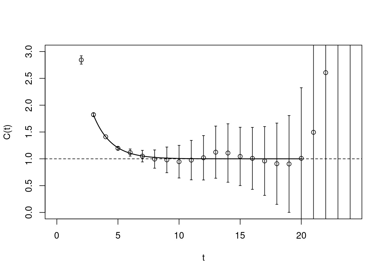
In such a plot all the data points should fluctuate around one. This matrixfit gives as a result \(E =0.334(60)\).
Effective Masses
Similaryly, effective masses \[ M_\mathrm{eff}\ =\ -\log\frac{C(t)}{C(t+1)} \] can be computed and bootstrapped as follows
pc1.effectivemass <- fit.effectivemass(cf=bootstrap.effectivemass(cf=pc1),
                                       t1=5, t2=20)
plot(pc1.effectivemass, col="red", pch=21, ylim=c(0,1),
     xlab="t", ylab="Meff")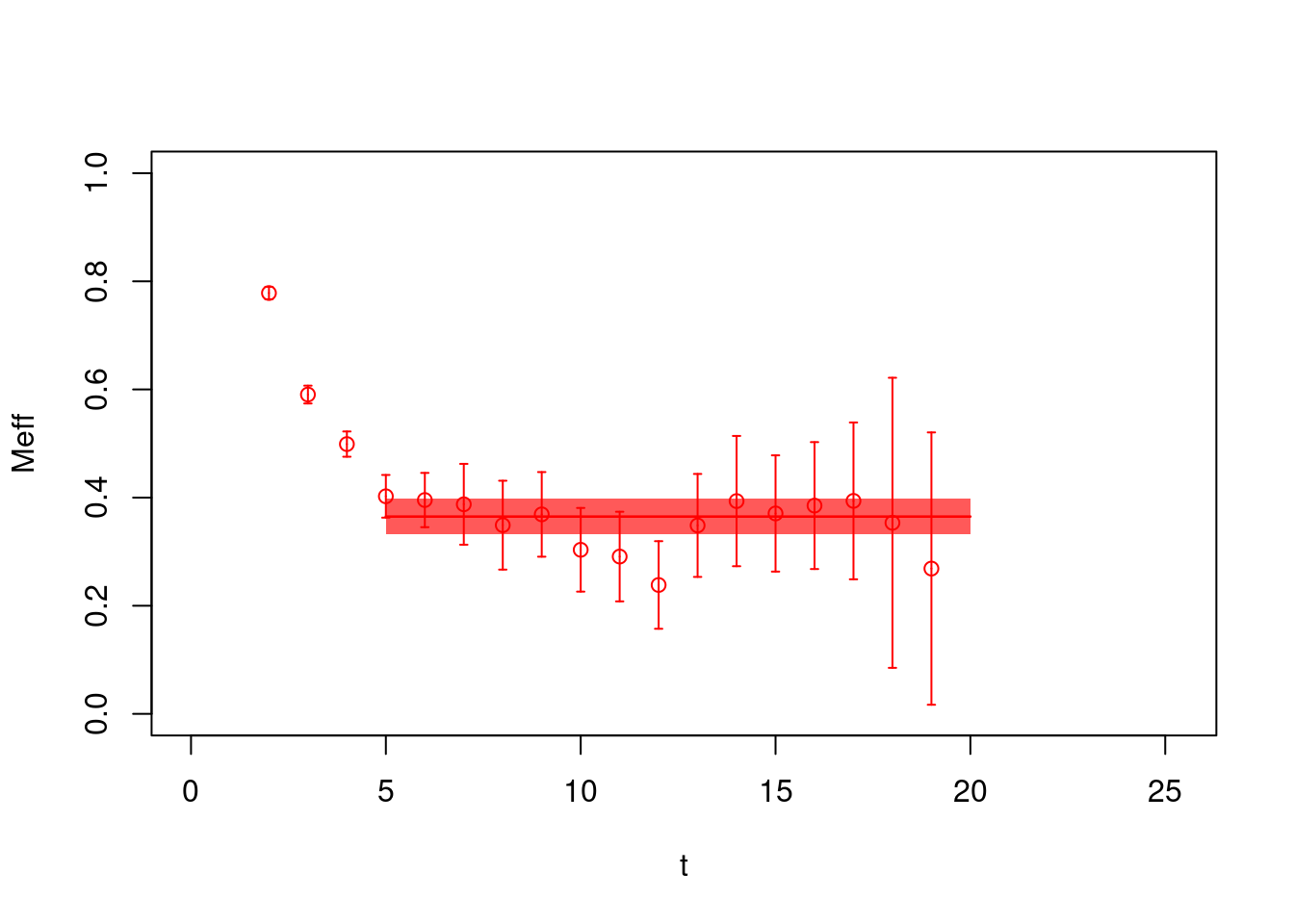
From the fit to the effective masses we obtain in this case \(E =0.365(33)\).
References
Fischer, Matthias, Bartosz Kostrzewa, Johann Ostmeyer, Konstantin Ottnad, Martin Ueding, and Carsten Urbach. 2020. “On the generalised eigenvalue method and its relation to Prony and generalised pencil of function methods.” Eur. Phys. J. A 56 (8): 206. https://doi.org/10.1140/epja/s10050-020-00205-w.
Lüscher, Martin, and Ulli Wolff. 1990. “How to Calculate the Elastic Scattering Matrix in Two-dimensional Quantum Field Theories by Numerical Simulation.” Nucl. Phys. B 339: 222–52. https://doi.org/10.1016/0550-3213(90)90540-T.
Michael, Christopher, and I. Teasdale. 1983. “Extracting Glueball Masses from Lattice QCD.” Nucl. Phys. B 215: 433–46. https://doi.org/10.1016/0550-3213(83)90674-0.